Scaling Laws, Carefully
Ch01.087 Scaling Laws, Carefully
📊 Level ⭐ | 6.4KB |
entities/posts-2026-06-24-scaling-laws.md
Scaling Laws, Carefully
Published Time: 2026-06-24T00:00:00Z
Markdown Content: Scaling laws are one of the most critical empirical findings in deep learning. The observation is simple in form: the training loss decreases predictably as we scale up model size , dataset size , and compute , following a power-law curve, which appears as a straight line on a log-log plot. We can view scaling laws as a framework for describing the relationship between compute, loss, model size and data; at its core, it is about how to allocate precious compute optimally between and .
This predictability makes scaling laws highly valuable in practice. A common workflow is to fit scaling laws on a handful of small runs and then extrapolate to estimate the token and compute requirements for larger models.
| Symbol | Note |
|---|---|
| $N$ | Model size, measured in parameter count. |
| $D$ | Training dataset size, usually measured in token count. |
| $C$ | Training compute in FLOPs. As a useful approximation, $C \approx 6 N D$ (Kaplan et al. 2020), where $2 N D$ accounts for the forward pass and $4 N D$ for backpropagation. |
| $E$ | Irreducible loss |
| $L , \hat{L} \left(\right. . \left.\right)$ | Test loss / test loss prediction function; can also refer to training loss, since they are strongly correlated. |
| $\epsilon$ | Generalization error. |
Early days: ML loss predictability
The predictability of generalization error with scale had already been investigated before scaling laws became a mainstream concept.
Amari et al. (1992) derived four types of learning curves using a Bayesian approach and the annealed approximation.
- Deterministic learning algorithm, noiseless data, one unique solution: , where is some constant.
- Deterministic learning algorithm, noiseless data, multiple equivalent solutions: ; the learning is faster with each new data point, because the model only learns the optimal manifold of parameters, instead of finding the single solution point.
- Deterministic learning algorithm, noisy data: ; noises in data make learning harder.
- Stochastic learning algorithm, noisy data: ; here the irreducible loss is the residual error that a stochastic learner cannot reduce further, for example when the model runs out of capacity on large data. All four types of learning curves follow a power law:
where can be 0 and . Although their theoretical setup is based on a simplified binary classification task, it points in a useful direction for building empirical ML loss prediction models.
One of the earliest empirical studies by Hestness et al. (2017) explained the relationship between generalization error, model size and data. For a given training data size, they identified the best-fit model size via grid search and then plotted loss against training dataset size. Across four different domains in deep learning (neural machine translation, image classification, language modeling, and speech recognition), a recurring pattern was observed where:
- Generalization error scales as a power law across a set of factors (e.g. data size).
- Model improvements shift the error curve but do not seem to affect the power-law exponent.
- Interestingly, architecture changes the offset () of the power-law fit but does not change the exponent (). The slope of the power law appears to be a property of the problem domain rather than the model architecture.
- The number of model parameters needed to fit a dataset of size also scales as a power law.
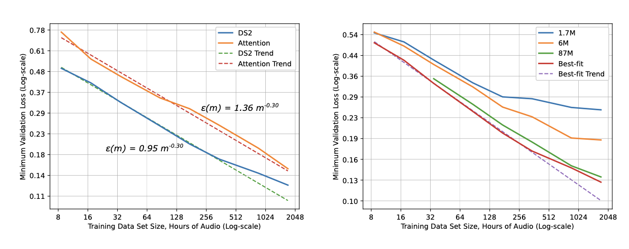
Learning curves for (Left) Deep-Speech-2 (DS2) and attention speech model and for (Right) DS2 models of various sizes. The losses of small models plateau when training data becomes large. (Image source: Hestness et al. 2017)
A conceptual illustration breaks the learning curve into three stages. In the small-data region, when there are not enough learning signals, the model performs only slightly better than random guessing. In the middle (“power-law region”), we observe a power-law relationship between loss, data, and model size. The final irreducible-error region can be attributed to factors such as noise in the data.
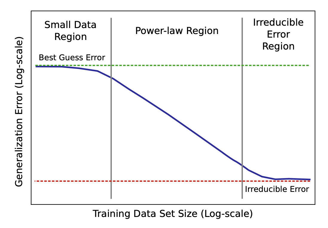
Illustration of power-law learning curve phases. (Image source: Hestness et al. 2017)
Rosenfeld et al. (2020) pushed this further by trying to model error as a joint function of both model size and data size , across a diverse set of architectures (ResNet, WRN, LSTM, Transformer) and optimizers (Adam, SGD variants). Empirically they observed that, holding one axis fixed, the error decays as a power law in the other:
which can be combined into a joint form:
where are scalar constants and is not dependent on either or .
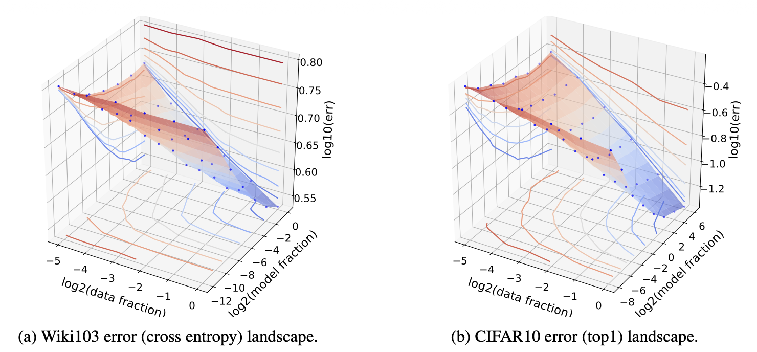
A 3D contour plot of data size, model size and generalization error in log-log-log scale. Blue dots are derived from empirical experiments and the surface is a linear interpolation between blue dots. (Image source: Rosenfeld et al. 2020)
Thus, they can build a prediction model in the form of a simple parametric function with to predict the expected loss for > certain thresholds by only training on a set of smaller training configs, < certain thresholds.
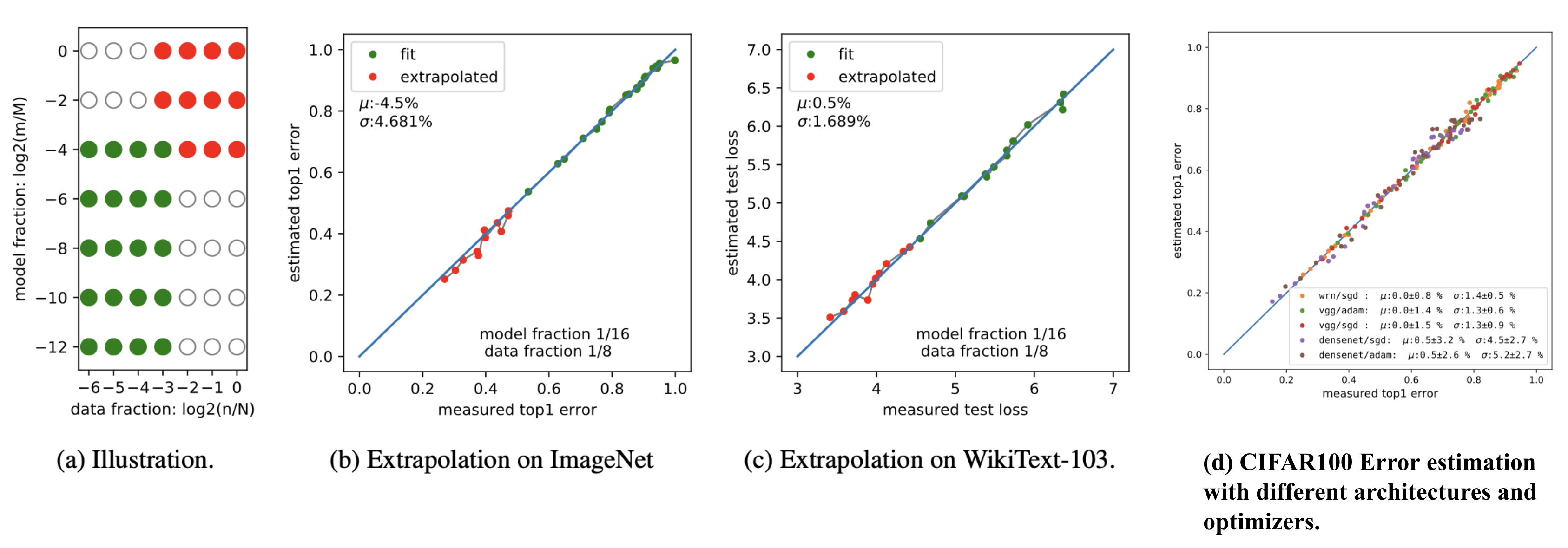
Fitting the parametric error model on small-scale configurations and extrapolating to larger model/data regimes: (a) Illustration of the experiment setup; Experiment results on (b) ImageNet, (c) WikiText-103 and (d) CIFAR100 Error estimation with three architectures (WRN, VGG, DenseNet) and two optimizers (SGD, Adam). (Image source: Rosenfeld et al. 2020)
Side note: These early works lean on
→ 原文存档